
AI and Machine Learning Concepts - Part 1
AI Product Management: Statistical Inference, Supervised Learning, Unsupervised Learning, Ensemble Models, and Reinforcement Learning

Dear readers,
Thank you for being part of our growing community. Here’s what’s new this today,
AI Product Management:
AI and Machine Learning Concepts - Part 1 (Statistical Inference, Supervised Learning, Unsupervised Learning, Ensemble Models, and Reinforcement Learning)
Note: This post is for our Paid Subscribers, If you haven’t subscribed yet,
Table of Contents:
The Machine Learning Landscape
Statistical Inference in Machine Learning
Supervised Learning
Classification Algorithms
k-Nearest Neighbors (kNN)
Logistic Regression
Naive Bayes
Decision Tree
Support Vector Machine (SVM)
Regression Algorithms
Linear Regression
Polynomial Regression
Lasso Regression (L1 Regularization)
Ridge Regression (L2 Regularization)
Unsupervised Learning
Clustering Algorithms
k-Means Clustering
DBSCAN (Density-Based Spatial Clustering)
Fuzzy C-Means
Mean-Shift Clustering
Pattern Search (Association Rule Mining)
Apriori Algorithm
ECLAT (Equivalence Class Transformation)
FP-Growth (Frequent Pattern Growth)
Dimensionality Reduction
PCA (Principal Component Analysis)
LDA (Linear Discriminant Analysis)
Other Dimensionality Reduction Techniques
Ensemble Models
Bagging (Bootstrap Aggregating)
Random Forest
Boosting
Stacking (Stacked Generalization)
Reinforcement Learning
Q-Learning
Deep Q-Network (DQN)
SARSA (State-Action-Reward-State-Action)
A3C (Asynchronous Advantage Actor-Critic)
Genetic Algorithm
[Important] How to Choose the Right Algorithm?
Introduction: The Machine Learning Landscape
Machine Learning (ML) is a branch of Artificial Intelligence (AI) where systems learn patterns from data and improve their performance without being explicitly programmed for every scenario. Rather than writing rules by hand, you feed data into an algorithm and let it discover the rules on its own.
Real-World Analogy
Think of ML like teaching a child to recognize animals. You do not give the child a rulebook with 10,000 rules. Instead, you show them hundreds of pictures of cats and dogs. Over time, the child learns to tell them apart on their own, even when they see a breed they have never encountered before. That is exactly how machine learning works.
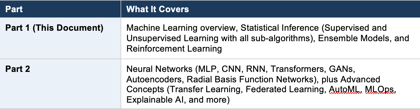
The ML ecosystem can be organized into several major branches. This two-part guide covers every concept from the taxonomy map, organized for easy reference:
Statistical Inference in Machine Learning
Statistical Inference is the process of drawing conclusions about a population based on sample data. In machine learning, this translates to training a model on a dataset (the sample) so it can make predictions or decisions about new, unseen data (the population). Almost all traditional ML algorithms fall under this umbrella.
PM Example
Your company has 50,000 users. You cannot manually study each one. Instead, you analyze behavioral data from a sample of 5,000 users and build a model that predicts churn risk for all 50,000. That is statistical inference in action: using a sample to draw conclusions about the whole.
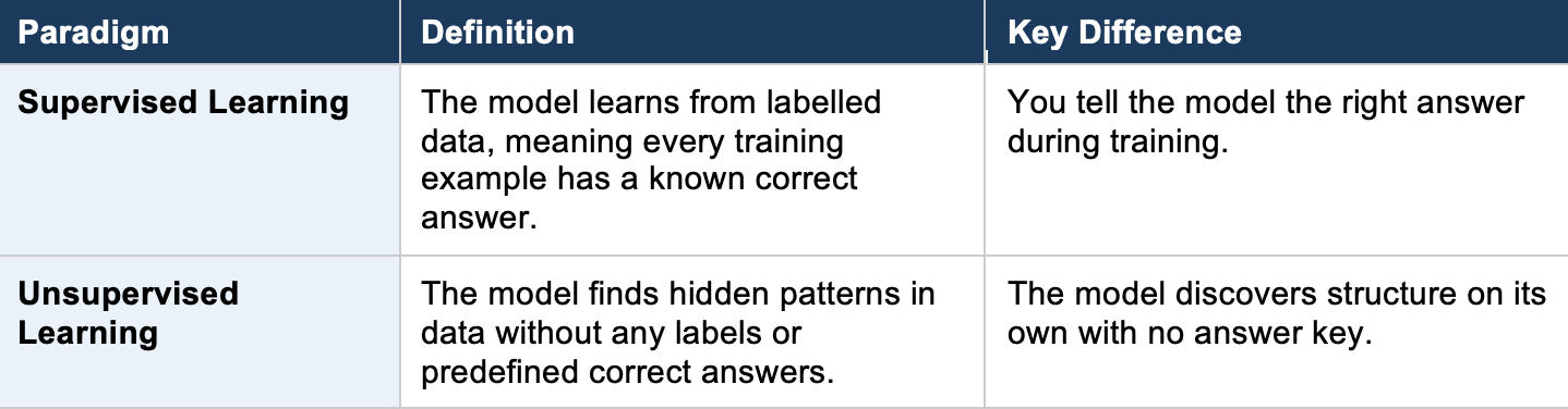
Statistical inference in ML divides into two major paradigms:
3. Supervised Learning
Supervised Learning is the most widely used form of machine learning. You provide the algorithm with input-output pairs (labeled data), and it learns a mapping function from inputs to outputs. Once trained, the model can predict outputs for new, unseen inputs.
Everyday Analogy
Imagine a student studying for an exam with a textbook that has questions and answers in the back. The student practices by reading each question, attempting an answer, then checking the correct answer to learn from mistakes. After enough practice, the student can answer new questions they have never seen before. That is supervised learning.
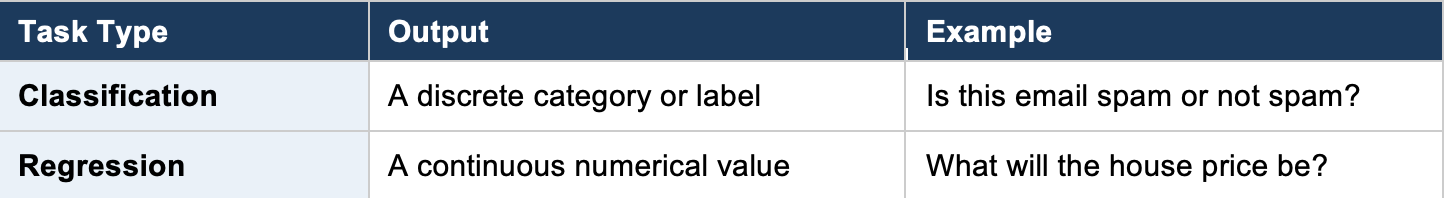
Supervised learning divides into two task types:
4. Classification Algorithms
Classification is the task of predicting which category or class an input belongs to. The model learns decision boundaries from labeled training data, then uses those boundaries to classify new data points.
4.1 k-Nearest Neighbours (kNN)
What it is: kNN is one of the simplest ML algorithms. It classifies a new data point by looking at the ‘k’ closest data points in the training set and assigning the majority class among those neighbors. It does not build an internal model during training; instead, it stores the entire dataset and makes decisions at prediction time.
PM Example: Customer Segmentation
You want to classify a new user as ‘high-value’ or ‘low-value.’ kNN looks at the 5 most similar existing users (based on features like session duration, purchase frequency, and support tickets). If 4 out of 5 neighbors are ‘high-value,’ the new user gets classified as high-value. It is like asking: ‘Who are the 5 people most like this new user, and what category do they fall into?’
When to Use kNN
Best for small to medium datasets where interpretability matters. Performs poorly on very large datasets because it must compare every new point against all training points. Also struggles with high-dimensional data (many features).
4.2 Logistic Regression
What it is: Despite its name, Logistic Regression is a classification algorithm, not a regression one. It predicts the probability that an input belongs to a particular class by fitting data to a logistic (S-shaped) curve. If the probability exceeds a threshold (typically 0.5), the input is classified as positive; otherwise, negative.
PM Example: Churn Prediction
You want to predict whether a customer will cancel their subscription next month. Logistic regression takes inputs such as login frequency, support tickets filed, days since last purchase, and feature usage. It outputs a probability, say 0.78 (78%). Since this exceeds your 0.5 threshold, you classify this customer as ‘likely to churn’ and trigger a retention campaign.
4.3 Naive Bayes
What it is: Naive Bayes is a family of probabilistic classifiers based on Bayes’ Theorem. It is called ‘naive’ because it assumes that all features are independent of each other, which is rarely true in practice but still produces surprisingly good results. It calculates the probability of each class given the input features and picks the most probable class.
PM Example: Spam Filtering
Your product has an in-app messaging system. Naive Bayes examines words in each message. It knows from training data that words like ‘free,’ ‘winner,’ and ‘click now’ appear frequently in spam. When a new message arrives containing these words, it calculates the probability of spam vs. not-spam and classifies accordingly. Gmail’s early spam filter used a version of this approach.
4.4 Decision Tree
What it is: A Decision Tree splits data into branches based on feature values, creating a tree-like structure of decisions. At each node, the algorithm chooses the feature that best separates the data (using metrics like Gini impurity or information gain). You follow the branches from root to leaf to arrive at a prediction.
PM Example: Feature Prioritization
Imagine deciding whether a feature request should be prioritized. The decision tree might ask: ‘Is the request from an enterprise customer?’ If yes, ‘Does it affect retention?’ If yes, ‘Priority: High.’ If no, ‘Does it affect more than 100 users?’ and so on. Each question splits the data until you reach a final decision. This mirrors how PMs often think through prioritization frameworks.
4.5 Support Vector Machine (SVM)
What it is: SVM finds the best hyperplane (a decision boundary) that separates data points of different classes with the maximum margin. The ‘support vectors’ are the data points closest to this boundary. SVM can also handle non-linearly separable data by using a ‘kernel trick’ that maps data into higher dimensions where a linear boundary becomes possible.
PM Example: Sentiment Classification
You are building a feature that classifies user reviews as positive or negative. SVM plots each review (represented as numerical features derived from text) in a multi-dimensional space and draws a boundary that best separates positive from negative reviews. New reviews are classified based on which side of the boundary they fall on.
5. Regression Algorithms
Regression is the task of predicting a continuous numerical value rather than a discrete category. The model learns the relationship between input features and a numerical target variable.
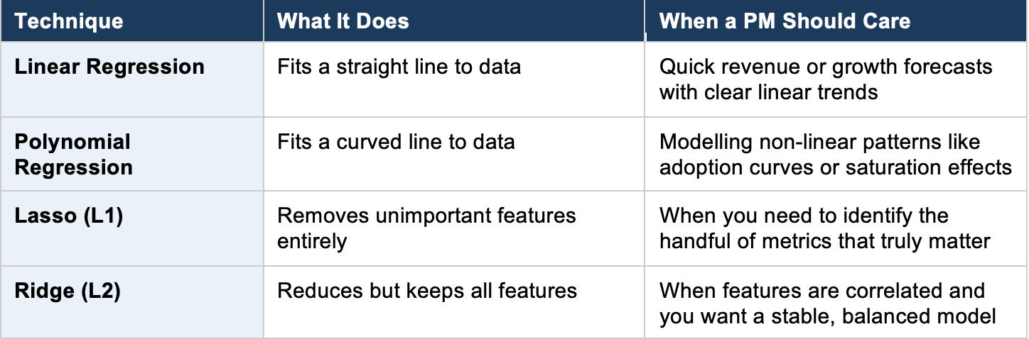
5.1 Linear Regression
What it is: Linear Regression is the simplest regression algorithm. It assumes a straight-line (linear) relationship between inputs and the output. The algorithm finds the best-fitting line through the data points by minimizing the sum of squared errors between predicted and actual values.
PM Example: Revenue Forecasting
You want to predict next month’s revenue based on marketing spend. Linear regression finds the line that best fits your historical data. If the relationship is ‘Revenue = $50,000 + (3.2 x Marketing Spend),’ and you plan to spend $10,000 on marketing, the model predicts $82,000 in revenue. Simple, interpretable, and often a great starting point.
5.2 Polynomial Regression
What it is: Polynomial Regression extends linear regression by fitting a curved line instead of a straight one. It adds polynomial terms (squared, cubed, etc.) to capture non-linear relationships in data.
PM Example: User Growth Modeling
Your product’s user growth is not linear. It starts slow, accelerates during product-market fit, then plateaus as the market saturates. A straight line cannot capture this S-curve pattern. Polynomial regression fits a curve that reflects these phases, giving you more accurate growth projections for board presentations.
5.3 Lasso Regression (L1 Regularization)
What it is: Lasso (Least Absolute Shrinkage and Selection Operator) is linear regression with an L1 penalty that pushes some feature coefficients all the way to zero. This effectively performs feature selection, keeping only the most important variables in the model.
PM Example: Identifying Key Engagement Drivers
You track 50 user engagement metrics. Which ones actually matter for retention? Lasso regression will analyze all 50 and zero out the irrelevant ones, leaving you with perhaps 8 features that truly drive retention. This tells your team exactly where to focus product improvements.
5.4 Ridge Regression (L2 Regularisation)
What it is: Ridge Regression adds an L2 penalty that shrinks feature coefficients toward zero but never eliminates them entirely. It is useful when you have many correlated features and want to prevent any single feature from dominating the model.
PM Example: Pricing Optimization
You are modeling how different factors (competitor prices, seasonality, user demographics, feature usage) influence willingness to pay. Many of these factors correlate with each other. Ridge regression keeps all variables in the model but prevents overfitting by shrinking their influence, giving you a stable pricing model.
6. Unsupervised Learning
Unsupervised Learning works with unlabeled data. The model has no answer key. Instead, it discovers hidden structures, groupings, and patterns within the data on its own. This is invaluable when you do not know what you are looking for, or when labeling data is too expensive.
Everyday Analogy
Imagine walking into a room full of 200 strangers at a conference. Nobody is wearing name tags or department labels. Over time, you notice natural clusters: a group discussing code, another talking about design, a third group focused on sales metrics. You have just performed unsupervised learning: finding structure without labels.
Unsupervised learning includes three major sub-categories:
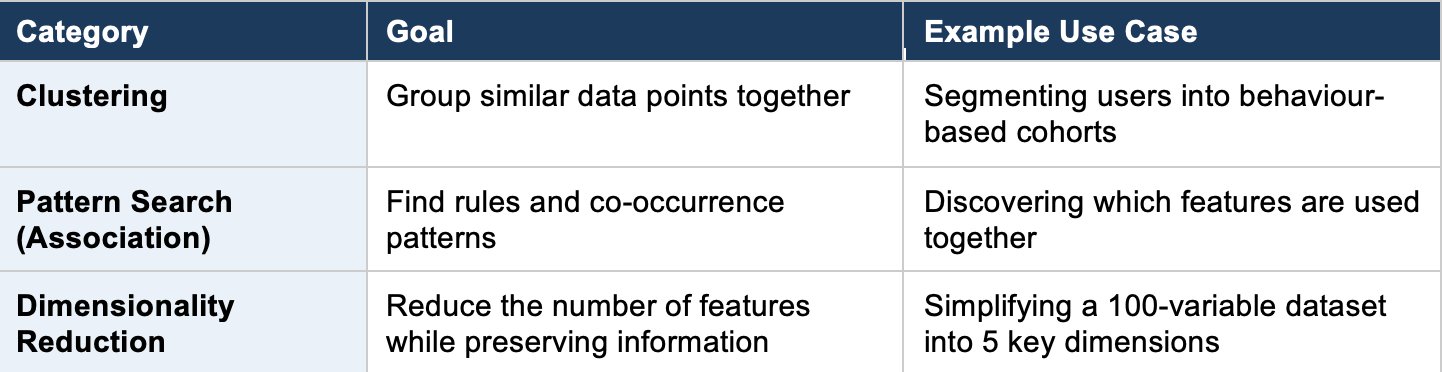
7. Clustering Algorithms
7.1 k-Means Clustering
What it is: k-Means divides data into ‘k’ clusters by repeatedly assigning each data point to the nearest cluster center (centroid) and then recalculating centroids. It continues until the assignments stabilize. You must choose the number of clusters (k) in advance.
PM Example: User Segmentation
You want to segment your 100,000 users into distinct groups for targeted messaging. You choose k=4. After running k-Means on engagement data, you discover four natural segments: Power Users (daily, heavy feature usage), Casual Browsers (weekly, light usage), Dormant Accounts (logged in once in 90 days), and New Explorers (joined recently, exploring features). Each segment gets a different retention strategy.
7.2 DBSCAN (Density-Based Spatial Clustering)
What it is: DBSCAN groups together data points that are closely packed (high density) and marks points in low-density regions as outliers. Unlike k-Means, you do not need to specify the number of clusters in advance. It finds clusters of arbitrary shapes and naturally identifies noise.
PM Example: Fraud Detection
You are analyzing transaction patterns. Most transactions cluster into normal behavior groups. DBSCAN identifies small, isolated clusters and individual outlier points that do not fit any group. These outliers are your fraud candidates. k-Means would have forced these anomalies into normal clusters, hiding the signal.
7.3 Fuzzy C-Means
What it is: Unlike k-Means where each point belongs to exactly one cluster, Fuzzy C-Means allows each point to belong to multiple clusters with different degrees of membership. A data point might be 70% Cluster A and 30% Cluster B.
PM Example: Content Recommendation
A user who watches both action movies and documentaries should not be forced into a single genre preference. Fuzzy C-Means would assign them 60% ‘action enthusiast’ and 40% ‘documentary lover,’ enabling your recommendation engine to suggest content from both categories proportionally.
7.4 Mean-Shift Clustering
What it is: Mean-Shift is a sliding-window-based algorithm that moves each data point toward the densest area of data points (the mean of the local neighborhood). Points that converge to the same location form a cluster. Like DBSCAN, it does not require specifying the number of clusters.
PM Example: Geographic Demand Analysis
You are launching a delivery service and want to identify hotspot zones without pre-deciding how many zones to create. Mean-Shift analyzes order locations and naturally identifies high-density demand clusters: downtown business districts, university areas, and suburban neighborhoods, each becoming a service zone.
8. Pattern Search (Association Rule Mining)
Association Rule Mining discovers interesting relationships and co-occurrence patterns in datasets. The classic application is market basket analysis: finding which items are frequently purchased together.
